 Honeycomb-Surfels:
Abstract
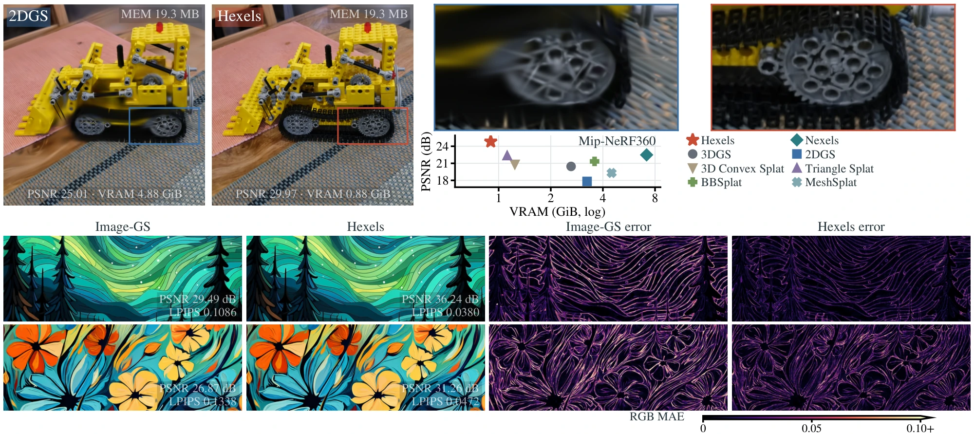
Novel view synthesis and 3D reconstruction have advanced rapidly with radiance fields and splatting, yet their memory and computational demands limit their use in resource-constrained settings. We introduce Hexels: novel planar hexagonal surface elements with a first-order spatial color field for efficient 3D scene and 2D image representation. Hexels exploit locally planar regions with smoothly varying appearance using fewer, larger primitives. Their hexagonal support provides an area- and boundary-efficient domain, while the local color field captures appearance variation within each primitive. Across 34 scenes, Hexels improve PSNR over memory-matched 2DGS by 4.53–7.38 dB across datasets while requiring lower training VRAM. We further ablate Hexels by showing that per primitive, Hexels outperform 2DGS by upto 4.74 dB while using lower training VRAM and having 2.31× faster FPS. Even in unconstrained settings, Hexels offers complementary quality-memory trade-offs. For efficient 3D surface reconstruction, Hexels reduce error by 28.9% compared with memory-matched 2DGS across 15 DTU scans. On 6 Tanks and Temples surface scenes, Hexels achieves the highest mean F1 among compared methods (34.38%, versus 31.72% for 2DGS). We further also show that Hexels, as a general primitive, improves 2D image representation over Image-GS. Hexels push the Pareto frontier on the quality-efficiency trade-off of surface-aligned primitives.
Method
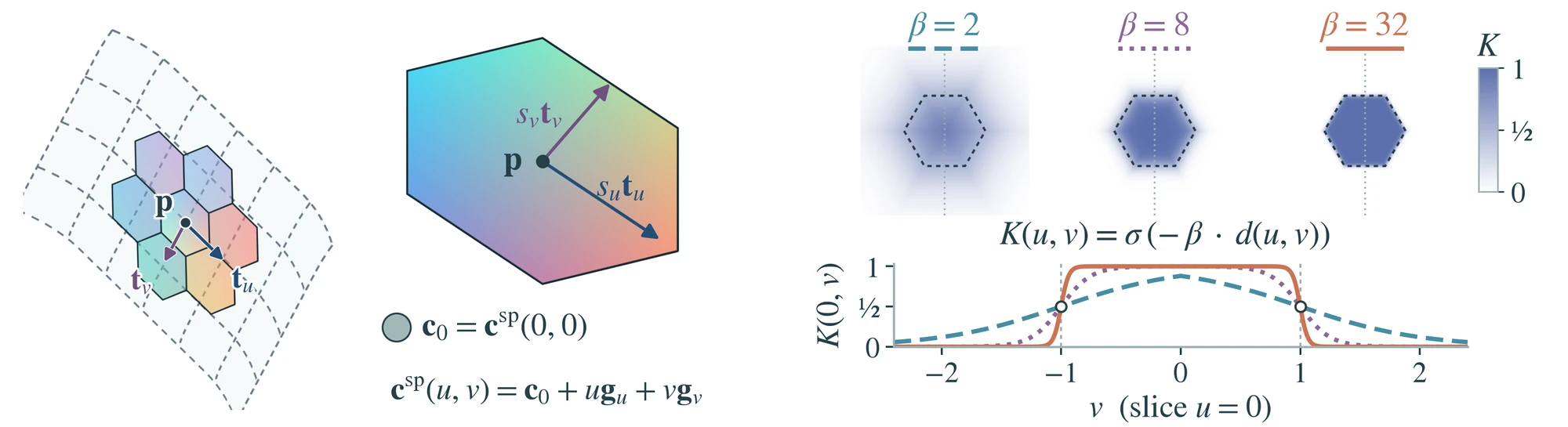
Each Hexel places its local coordinates \((u,v)\) in 3D through its center \(\mathbf{p}\), unit tangents \(\mathbf{t}_u,\mathbf{t}_v\) and scales \(s_u,s_v\), and its color changes linearly along them:
Where a pixel's ray meets the plane, the Hexel's opacity \(o\) times its soft hexagonal support \(K\), capped at 0.99, gives its alpha \(\alpha=\min\{o\cdot K,\,0.99\}\), and colors are blended front to back as in 2DGS. Because the color varies across each patch, fewer, larger Hexels can cover regions whose appearance changes smoothly. V1 uses this spatial color alone, 20 learned numbers per Hexel, while V2 and V3 add an RGB offset that depends on the viewing direction, for 29 and 65 numbers.
In the paper: Figure 2 and Section 3, Eqs. (1) to (4). The parameter counts and appearance variants are in Appendix A, the rasterizer in Appendix B.
What the primitives look like
Drag the crosshair to compare the renders (top) and the primitives (bottom) of Hexels and a Gaussian method, 3DGS or 2DGS, with every primitive drawn in a random color.
Novel view synthesis
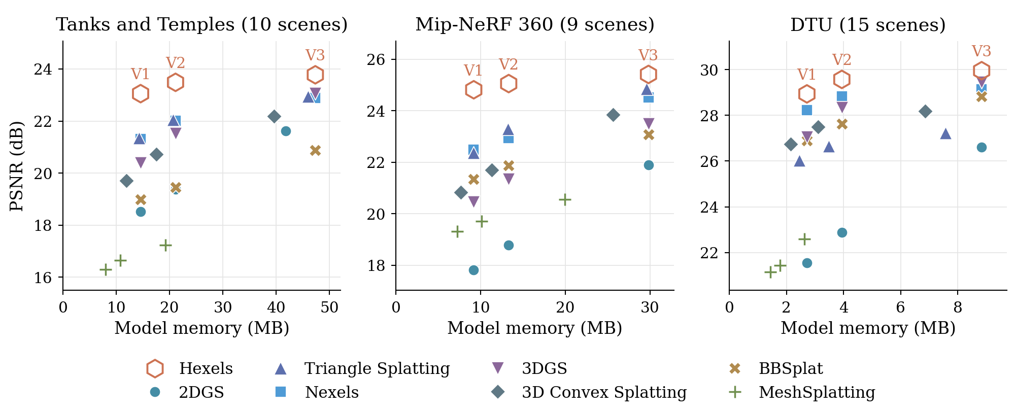
Equal memory is the paper's primary setting: in each scene, every baseline is trained within the model memory of fixed Hexels V1, so all methods share one storage budget. Pick a scene and a method for each side and drag the divider to compare; pause the video to see synchronized close-ups of all eight methods.
Equal primitives compares the primitives themselves: every baseline is capped at the scene's SfM point count, the population of fixed Hexels V3, so all methods share one primitive budget. Pick a scene and a method for each side and drag the divider to compare; pause the video to see synchronized close-ups of all eight methods.
Native settings lift both limits: Hexels V3 (densified) and eight baselines train with their own population policies and no cap on model memory or primitive count. Pick a scene and a method for each side and drag the divider to compare; pause the video to see synchronized close-ups of all nine methods.
Quantitative results
Rendering quality against efficiency for Hexels and seven baselines. On Tanks and Temples, Hexels V3 (densified) reach 24.53 dB, above 2DGS (23.64 dB), Triangle Splatting (23.15 dB) and MeshSplatting (20.73 dB), and Hexels V2 keeps 23.49 dB in 21.12 MB. Averaged over the three datasets, Hexels V3 (densified) match 3DGS in PSNR (26.94 versus 26.93 dB) with less than half its model memory (152.26 versus 340.20 MB). Pick a dataset, a quality metric and an efficiency metric; hover over or tap a point for all of its numbers.
Quality at matched model memory
Hexels variants
Six Hexels models trained from the same COLMAP initialization: V1 (spatial color gradient), V2 (plus a linear view-dependent term) and V3 (plus degree-3 spherical harmonics), each with a fixed population or with densification. The grid plays all six along the same camera path. Densification adds the most on the large unbounded scenes (Mip-NeRF 360: 24.82 to 26.05 dB for V1, 25.41 to 26.52 dB for V3) and the least on DTU objects, where fixed V3 scores best (29.95 dB in 8.83 MB). Spherical harmonics improve every fixed population (Mip-NeRF 360: 24.82 to 25.41 dB; DTU: 28.94 to 29.95 dB), while densified V3 needs far more training memory (13.95 versus 2.75 GiB of peak VRAM for densified V2 on Mip-NeRF 360).
Surface reconstruction
Here we compare surface reconstruction quality of Hexels against 2DGS, Triangle Splatting and MeshSplatting. Chamfer distance (mm, lower is better) is used for evaluation on 15 DTU scans and F-score on 6 Tanks and Temples scenes (%, higher is better). On DTU, Hexels V3 with MVS initialization average 0.978 mm, behind unconstrained 2DGS (0.794 mm) but ahead of 2DGS matched to Hexels' memory (1.375 mm) or primitive count (1.449 mm), Triangle Splatting (1.124 mm) and MeshSplatting (1.662 mm). On Tanks and Temples Hexels gives the highest mean F-score, 34.38% against 31.72% for 2DGS.
Depth and normals
Expected depth and rendered normals of Hexels V3 (densified) for one held-out view per dataset. Depth is color-coded by inverse depth from red (near) to blue (far), and the camera-space normals \(\mathbf{n}\) (x right, y up, z toward the viewer) are shown as RGB \((\mathbf{n}+1)/2\).
Depth near far
Normals facing the camera facing right facing up no surface
2D image representation
The same primitive represents images directly in the image plane, without projection, opacity or depth ordering. On the 45-image Image-GS benchmark, with 10,000 primitives per image at the end of the fit, Hexels raise PSNR from 33.16 to 35.82 dB and lower LPIPS from 0.1372 to 0.0924 against Image-GS, with 5,100 instead of 10,000 iterations and 157 instead of 238 seconds of fitting. Hexels start from 20,000 primitives and prune down to 10,000 while fitting. Even constant-color Hexels, which store the same eight numbers per primitive as Image-GS, reach 34.16 dB.
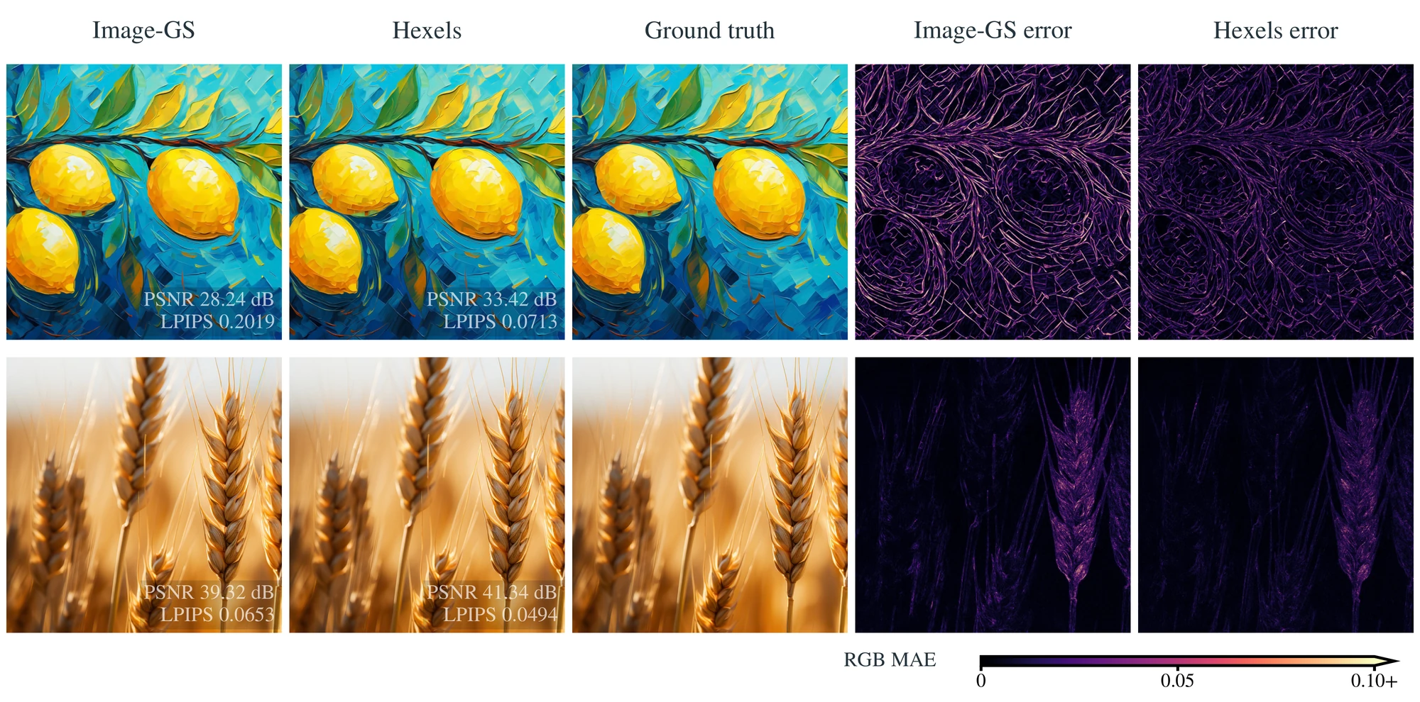
Image-GS benchmark, 45 images, with 10,000 primitives per image at the end of the fit. Constant-color Hexels store the same eight scalars per primitive as Image-GS. Bold marks the best value in each column, as in the paper.
| Method | PSNR ↑ | SSIM ↑ | LPIPS (AlexNet) ↓ | Iterations ↓ | Train (s) ↓ | Disk size (kB) ↓ |
|---|---|---|---|---|---|---|
| Image-GS | 33.16 | 0.9141 | 0.1372 | 10,000 | 238.40 | 292.175 |
| Hexels (constant) | 34.16 | 0.9208 | 0.1099 | 5,100 | 112.11 | 289.799 |
| Hexels | 35.82 | 0.9359 | 0.0924 | 5,100 | 157.07 | 551.174 |
BibTeX
@misc{kaushik2026honeycombsurfelscompacthexagonalprimitives,
      title={Honeycomb-Surfels: Compact Hexagonal Primitives for Efficient Scene Rendering and Reconstruction},
      author={Prakhar Kaushik and Soumava Paul and Alan Yuille},
      year={2026},
      eprint={2610.37668},
      archivePrefix={arXiv},
      primaryClass={cs.CV},
      url={https://arxiv.org/abs/2610.37668},
}